Understanding Linear Temporal Logic: Syntax, Semantics, and Model Checking

This is a summary of linear temporal logic lecture held by Reiner Hähnle at TU Darmstadt. Also this whole post has his slides as source.

Summary of Linear Temporal Logic Lecture

Introduction

In the lecture on linear temporal logic by Reiner Hähnle at TU Darmstadt, the process of formalizing real-world concepts into formal models was discussed. These models are described using formal languages, which provide the syntax for expressing the models. The syntax primarily consists of propositional logic and can also incorporate temporal logic and Promela syntax options to represent temporal properties and system behaviors. The semantics of the models are defined through transition systems, considering all possible runs denoted as σ.

Model Checking

The lecture delved into the topic of model checking and how it can be performed. In most cases, temporal logic involves translating negation into a Büchi automaton, while Promela syntax also transforms into a Büchi automaton. By combining both the temporal logic and Promela automata into a product automaton, it becomes possible to verify if there are any runs that are not accepted by the automaton.

Syntax, Semantics, and Calculus

Understanding the relationship between syntax, semantics, and calculus is essential in this context. Syntax formulas can be evaluated by determining their semantics, checking if they are “valid” or satisfy certain properties. The lecture emphasized the importance of ensuring soundness and completeness of the calculus used to derive the semantics. Propositional formulas and sequent calculus were highlighted as tools to reason about syntax and semantics. Additionally, SAT solvers with sequent calculus were mentioned as useful for checking the satisfiability of propositional formulas, aiding in model checking and analysis.

Completeness and Soundness

Soundness was explained as a property that guarantees the correctness of a logical system. In propositional logic, soundness establishes the logical connection between syntax and semantics, ensuring that derivable formulas are semantically valid.

Completeness, on the other hand, ensures that all valid formulas can be derived or proven within a logical system. It establishes that the proof system is comprehensive enough to capture all valid formulas and leaves no valid formula unproven or undecidable.

In conclusion, the lecture provided insights into the process of formalization, including the selection of formal languages, defining semantics, and employing calculus and analysis techniques to reason about the validity and completeness of models. The lecture highlighted the significance of propositional formulas, sequent calculus, and SAT solvers as valuable tools in this endeavor.

Propositional Logic

Propositional logic provides a formal language for expressing logical statements and reasoning about their truth values. It consists of a set of propositional variables and connectives that allow us to construct formulas. Here are the key components of propositional logic:

Propositional Variables

Propositional variables, denoted as P, Q, R, etc., represent atomic propositions or simple statements that can be either true or false. These variables serve as the building blocks for constructing more complex formulas.

Connectives

Propositional logic introduces several connectives to combine and manipulate propositions:

• Conjunction (∧): The conjunction of two formulas is true only if both formulas are true.

• Disjunction (∨): The disjunction of two formulas is true if at least one of the formulas is true.

• Negation (¬): Negation flips the truth value of a formula. It is used to express the opposite of a proposition.

• Implication (→): Implication represents the logical relationship between two formulas, stating that if the antecedent is true, then the consequent must also be true.

• Equivalence (↔): Equivalence indicates that two formulas have the same truth value. They are either both true or both false.

Formula Construction

Propositional formulas can be constructed by combining propositional variables and connectives according to the following rules:

1. Propositional variables and truth constants (true and false) are considered formulas.

2. If ϕ and ψ are formulas, then ¬ϕ (negation of ϕ), (ϕ ∧ ψ) (conjunction of ϕ and ψ), (ϕ ∨ ψ) (disjunction of ϕ and ψ), (ϕ → ψ) (implication from ϕ to ψ), and (ϕ ↔ ψ) (equivalence between ϕ and ψ) are also formulas.

3. Any other expressions are not considered formulas.

These rules allow us to create complex formulas by combining simpler ones using the propositional variables and connectives.

Valuation

In propositional logic, a valuation assigns truth values (T or F) to propositional formulas based on a given interpretation or truth assignment. The valuation function extends the interpretation to all propositional formulas. Let’s examine how the valuation function assigns truth values to different types of formulas:

Atomic Formulas

For atomic formulas or propositional variables (pi), the valuation function retrieves the truth value assigned to the variable by the interpretation I. In other words, valI(pi) is equal to I(pi).

Truth Constants

The valuation function assigns specific truth values to the truth constants:

• valI(true) = T
• valI(false) = F

Connectives

The valuation function for different connectives is as follows:

• Negation (¬): valI(¬ϕ) = T if valI(ϕ) = F; valI(¬ϕ) = F otherwise.

• Conjunction (∧): valI(ϕ ∧ ψ) = T if valI(ϕ) = T and valI(ψ) = T; valI(ϕ ∧ ψ) = F otherwise.

• Disjunction (∨): valI(ϕ ∨ ψ) = T if valI(ϕ) = T or valI(ψ) = T; valI(ϕ ∨ ψ) = F otherwise.

• Implication (→): valI(ϕ → ψ) = T if valI(ϕ) = F or valI(ψ) = T; valI(

ϕ → ψ) = F otherwise.

• Equivalence (↔): valI(ϕ ↔ ψ) = T if valI(ϕ) = valI(ψ); valI(ϕ ↔ ψ) = F otherwise.

By applying the valuation function to propositional formulas, we can determine their truth values based on the assigned interpretation.

Note: While the provided text mentions a specific concrete syntax used in the textbook “Spin” resembling C-like notation, the general principles and rules of propositional logic remain the same. The specific notation may vary in different contexts or tools, but the fundamental concepts and syntax rules of propositional logic remain consistent.

Satisfying Interpretation, Consequence Relation

Let’s discuss the concepts of satisfying interpretation and consequence relation in propositional logic.

Satisfying Interpretation: An interpretation I is said to satisfy a propositional formula ϕ (written as I |= ϕ) if the truth value assigned to ϕ by the valuation function valI is T. In other words, if valI(ϕ) = T, then the interpretation I satisfies the formula ϕ.

Consequence Relation: The consequence relation relates a set of formulas Γ to a formula ϕ. We write Γ |= ϕ to indicate that ϕ follows or is a logical consequence of Γ. The consequence relation holds if, for all interpretations I:

• If I satisfies every formula ψ in Γ (written as I |= ψ for all ψ ∈ Γ), then I also satisfies the formula ϕ (written as I |= ϕ).

In other words, ϕ follows from Γ if, under any interpretation that satisfies all formulas in Γ, ϕ is also satisfied. This can be expressed using set notation as follows:

{I | I |= ψ for all ψ ∈ Γ} ⊆ {I | I |= ϕ}

or in a more mathematical way:

\[\{\mathcal{I} \mid \forall \psi \in \Gamma, \mathcal{I} \models \psi\} \subseteq \{\mathcal{I} \mid \mathcal{I} \models \phi\}\]

Satisfiability: A formula ϕ is considered satisfiable if there exists an interpretation I that makes ϕ true. In other words, there is at least one assignment of truth values to the propositional variables in ϕ that results in the entire formula evaluating to true. This means that there is a way to satisfy the conditions and make the formula consistent with the given interpretation. If even a single interpretation satisfies ϕ, then it is considered satisfiable.

Validity: On the other hand, a formula ϕ is called valid if every interpretation, without exception, satisfies ϕ. In other words, regardless of how we assign truth values to the propositional variables, the formula always evaluates to true. When we write “⊨ ϕ,” we mean that every possible interpretation leads to ϕ being true. Valid formulas express statements that are universally true, regardless of the specific circumstances or values assigned to the variables.

Formalisation of Promela in Propositional Logic

Consider the following Promela program P:

// Program P
byte n ;
active proctype [2] p () {
    n = 0;
    n = n + 1
}

In this formalization, we can define interpretations based on the state and program counter. The eight bits representing variable ‘n’ can take any possible value. A process cannot be simultaneously present at two different positions. If neither process 0 nor process 1 is at position 5, then ‘n’ is equal to zero.

To express properties of program P, we can define a formula ϕP using propositional logic that encompasses the relevant conditions and constraints:

ϕP := ((PC03 ∧ ¬PC04 ∧ ¬PC05) ∨ ...) ∧
       ((¬PC05 ∧ ¬PC15) ⇒ (¬N0 ∧ ... ∧ ¬N7)) ∧ ...

This formula ϕP captures the state and program counter conditions of program P. It represents a conjunction of various atomic propositions related to the program’s execution states and variables.

To express specific properties, such as whether ‘n’ will become greater than 0 eventually or ‘n’ changes infinitely often, we need to involve state change properties. This requires a more expressive logic than propositional logic, namely linear temporal logic (LTL). LTL allows us to reason about temporal properties and specify temporal patterns and behaviors.

In summary, while propositional logic is suitable for capturing static properties and constraints, the formalization of dynamic properties and temporal behaviors requires the use of more expressive logics like linear temporal logic.

Linear Temporal Logic

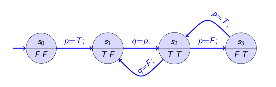[Kripke Structure Source: Rainer Hähnle]

In the context of Kripke structures, the following statements apply:

• Each state s_j in the program is associated with its own interpretation of the propositional variables, denoted as I_j.
• The values of variables are conventionally listed in ascending lexicographic order.
• Computations, also known as runs, are represented as infinite paths that traverse through different program states.
• It is important to note that the concept of “infinite” does not impose a restriction, as finite runs can also occur, where the computation ends at a final state.
• In general, there is a possibility of infinitely many distinct runs, each with its own sequence of states and variable interpretations.

It can be observed that the runs of a Promela program can be viewed as runs of a suitable transition system, drawing a parallel between the behavior of the program and the behavior of the corresponding transition system.

The syntax of this extended propositional logic is based on the propositional signature and syntax. In addition to the standard propositional connectives, we have three new connectives:

• Always (□): If ϕ is a formula, then □ϕ is also a formula. The “Always” connective represents a property that holds for every point in a run or trace.

• Sometimes (♢): If ϕ is a formula, then ♢ϕ is also a formula. The “Sometimes” connective represents a property that holds for at least one point in a run or trace.

• Until (U): If ϕ and ψ are formulas, then ϕ Uψ is also a formula. The “Until” connective represents a property that holds until another property becomes true. It specifies that ϕ holds at every point in a run until ψ becomes true, including the point where ψ becomes true.

Concrete Syntax:

The concrete syntax for this extended propositional logic is often represented using the textbook Spin notation. The connectives are written as follows:

• Always: [ ]
• Sometimes: <>
• Until: U

These concrete syntax notations are commonly used in Spin, a popular tool for model checking and verification.

In propositional logic, a propositional formula is evaluated relative to a single interpretation, which assigns truth values to the propositional variables in the formula. The interpretation provides a consistent assignment of truth values, allowing us to determine the overall truth value of the formula. Each propositional variable in the formula is mapped to either true or false according to the interpretation.

On the other hand, in temporal logic, a temporal formula is evaluated relative to a sequence of interpretations. Instead of a single interpretation, we consider a sequence or series of interpretations, which represent different points or moments in time. Each interpretation in the sequence corresponds to a specific state or configuration of the system being analyzed. By evaluating the formula at each point in the sequence, we can capture temporal aspects such as the progression of time, state transitions, and the behavior of the system over time.

“If σ = s0 s1 · · · , then σ

i denotes the suffix si si+1 · · · of σ.”

The validity of a temporal formula in temporal logic depends on the runs or sequences of states, denoted as σ = s0 s1 · · ·. Each state in the sequence is assigned an interpretation, following the convention that the interpretation in state s_j is denoted as I_j.

The validity relation is defined as follows:

• σ |= p: The temporal formula p is valid in the run σ if and only if the proposition

• p is true in the initial state I_0 of σ. This means that the interpretation I_0 assigns the truth value “true” to the proposition p.

• σ |= ¬ϕ: The negation of the temporal formula ϕ is valid in the run σ if and only if ϕ is not valid in the same run. This is denoted as “not σ

  = ϕ,” indicating that the formula ϕ is not true in the run σ.

• σ |= ϕ ∧ ψ: The conjunction of two temporal formulas ϕ and ψ is valid in the run σ if and only if both ϕ and ψ are valid in the same run. This requires that the run σ satisfies both ϕ and ψ simultaneously.

• σ |= ϕ ∨ ψ: The disjunction of two temporal formulas ϕ and ψ is valid in the run σ if and only if at least one of ϕ or ψ is valid in the same run. This means that the run σ satisfies either ϕ or ψ, or both.

• σ |= ϕ → ψ: The implication of two temporal formulas ϕ and ψ is valid in the run σ if and only if either ϕ is not valid in the run σ, or ψ is valid in the same run. This captures the condition that if ϕ is not satisfied, then the implication ϕ → ψ is automatically considered true.

For propositional formulas, the evaluation is done in the interpretation of the initial state σ_0 of the run σ.

Safety and Liveness

In temporal logic, safety and liveness properties are two important types of properties that can be expressed and analyzed.

Safety Properties:

Safety properties are expressed using always-formulas (□ϕ) and they represent conditions where “something bad never happens.” These properties typically specify constraints or restrictions on system behavior to ensure safety or prevent undesirable situations. Checking safety properties requires examining the entire infinite run (not just the prefix) of the system, as they cannot be verified using a finite prefix of the run.

For example, consider the variable “mutex” that is true when two processes do not access a critical resource at the same time. The formula □mutex expresses the safety property that simultaneous access to the critical resource never happens.

Liveness Properties:

Liveness properties are expressed using sometimes-formulas (♢ϕ) and they represent conditions where “something good happens eventually.” These properties typically capture desired system behaviors that involve progress, reachability, or the eventual occurrence of certain events. Checking liveness properties can often be established by examining a finite prefix of the run, as they focus on the eventual occurrence of events (but it could happen that you need to check the whole run).

For example, consider the variable “s” that is true when a process delivers a service. The formula ♢s expresses the liveness property that the service is eventually provided.

Both safety and liveness properties play crucial roles in the analysis and verification of systems. Safety properties ensure that undesirable states or behaviors are avoided, while liveness properties ensure that desired events or behaviors eventually occur. By specifying and checking these properties, we can ensure the reliability, correctness, and desired behavior of complex systems.

Example:

σ |= □♢ϕ
"During run σ, the formula ϕ becomes true infinitely often"

Transition Systems

A transition system T = (S, Ini, δ, I) is a formal structure used to describe the behavior and dynamics of a system. It comprises the following components:

1. Set of states (S): This set includes all the possible states that the system can assume. Each state represents a specific configuration or snapshot of the system.

2. Set of initial states (Ini): Ini is a non-empty subset of the set of states (S) and represents the states from which the system can start its execution.

3. Transition relation (δ): The transition relation δ defines how the system moves from one state to another. It specifies the possible state transitions based on the current state. Typically, δ is represented as a subset of the Cartesian product of the set of states (S) with itself (S × S).

4. Labeling function (I): The labeling function I associates propositional interpretations with each state in the system. It provides additional information or labels associated with states, which can be used to express properties or conditions about the system’s behavior.

Example: Let’s consider a light switch system with two states: Off and On.

• Set of states (S): {Off, On} The system has two possible states: Off and On. These states represent the current state of the light switch, indicating whether the light is turned off or on.

• Set of initial states (Ini): {Off} The initial state of the system is Off, indicating that the light switch starts in the off position.

• Transition relation (δ):
  • (Off, On): If the light switch is in the Off state and a user toggles the switch, it transitions to the On state.
  • (On, Off): If the light switch is in the On state and a user toggles the switch, it transitions to the Off state.
• Labeling function (I):
  • I(Off) = {LightOff}: The Off state is labeled with the proposition “LightOff,” indicating that the light is turned off.
  • I(On) = {LightOn}: The On state is labeled with the proposition “LightOn,” indicating that the light is turned on.

Given a transition system T = (S, Ini, δ, I), we can analyze its behavior, properties, and the satisfaction of certain conditions using formal methods such as model checking and temporal logic.

Büchi Automaton

A Büchi automaton, also known as a ω-automaton, is a type of non-deterministic finite-state automaton designed to handle infinite inputs or infinite sequences of symbols.

A Büchi automaton consists of the following components:

1. Set of locations (Q): Q is a finite, non-empty set of states or locations that the automaton can be in. Each location represents a specific configuration of the automaton.

2. Set of initial/start locations (I): I is a non-empty subset of the set of locations (Q) and represents the starting states of the automaton. When the automaton begins its operation, it starts from one or more initial locations.

3. Set of accepting/final locations (F): F is a set of locations (F = {F1, . . . , Fn}) designated as accepting or final states. These states indicate that the automaton has reached a desirable condition or satisfied a specific property. In Büchi automata, the acceptance condition is defined using a Büchi acceptance condition, which requires visiting accepting states infinitely often.

4. Transition relation (δ): The transition relation δ specifies the possible state transitions of the automaton based on the current location and the input symbol. It is represented as a subset of the Cartesian product of the set of locations (Q) with the input alphabet

.

The primary purpose of a Büchi automaton is to recognize or accept infinite words or infinite sequences of symbols over the input alphabet. By defining the set of accepting locations and the transition relation, the automaton can determine if an input sequence satisfies the specified acceptance condition, such as visiting the accepting states infinitely often.

Büchi automata find applications in various areas, including formal verification, model checking, and formal languages theory. They are used to reason about the properties and behavior of systems that exhibit infinite or unbounded behavior, enabling analysis and verification of complex systems with temporal or infinite aspects.

Büchi Automaton Acceptance

In the context of Büchi automata, a run refers to an infinite word or sequence of symbols over the alphabet Σ, denoted as w = a0a1a2…ak…, where each ai represents a symbol from Σ.

A run is considered valid for a Büchi automaton if, starting from an initial location q0 in the set of locations Q, the transition relation δ allows transitioning from one state to another based on the corresponding input symbol. Specifically, for each position i in the run, if qi is the current location, then qi+1 must belong to δ(qi, ai) according to the transition relation.

An accepted run for a Büchi automaton is a run in which at least one accepting location f from the set of accepting locations F is visited infinitely often. This means that, as the automaton progresses along the run, it repeatedly reaches and stays in at least one accepting location, ensuring that the desired acceptance condition is met.

The language recognized by a Büchi automaton B, denoted as Lω(B), is defined as the set of all infinite words w ∈ Σω that correspond to accepted runs of the automaton B.

An ω-regular language is a language that can be recognized by a Büchi automaton. In other words, if there exists an automaton that accepts all the runs representing the language, then the language is said to be ω-regular. Büchi automata and ω-regular languages are fundamental concepts in formal languages theory, automata theory, and formal verification, particularly for reasoning about infinite or unbounded behaviors in systems.

Two important theorems related to Büchi automata and ω-regular languages are as follows:

1. The emptiness problem: It is decidable whether the accepted language Lω(B) of a Büchi automaton B is empty. This means that there exists an algorithm or procedure that can determine whether the language recognized by the Büchi automaton contains any words.

2. Closure properties: ω-regular languages exhibit closure properties. Specifically, if L1 and L2 are ω-regular languages, then their intersection L1 ∩ L2 and union L1 ∪ L2 are also ω-regular languages. Furthermore, if L is an ω-regular language, then its complement Σω\L (the set of all possible ω-words that are not in L) is also an ω-regular language.

It is important to note that non-deterministic Büchi automata are more expressive than deterministic ones when it comes to accepting ω-regular languages. Deterministic Büchi automata cannot accept all possible ω-regular languages, whereas non-deterministic Büchi automata have the capability to recognize any ω-regular language.

To construct a Büchi automaton that accepts runs satisfying an LTL formula ϕ (Linear Temporal Logic), a connection needs to be established between the LTL formula and the automaton’s alphabet.

In this context, the alphabet Σ of the Büchi automaton consists of all possible interpretations over a set of propositional variables P. Each interpretation corresponds to a state transition in the automaton.

For example, consider a simple set of propositional variables P = {r, s}. The alphabet Σ would then be 2P, representing all possible interpretations over P. In this case, Σ would consist of the following interpretations:

Σ = {∅, {r}, {s}, {r, s}}

To establish the connection between an interpretation and its corresponding state transition, an interpretation function Ia can be defined for each interpretation a ∈ Σ. For example:

I∅(r) = F

I∅(s) = F I{r}(r) = T, I{r}(s) = F

---

The interpretation function assigns truth values (T or F) to each propositional variable based on the given interpretation.

By constructing a Büchi automaton with the alphabet Σ and defining its state transitions based on the interpretation functions, it is possible to design an automaton that accepts runs satisfying the LTL formula ϕ. The automaton will transition between states based on the interpretations of the propositional variables, allowing for the determination of whether a run satisfies the formula or not.